Chapter 21 The Accuracy of Percentages
21.1 Chapter Notes
In the last chapter, we used a box model with known composition to reason about the expected values and standard errors of the sample. This chapter concerns the reverse: making inferences about a population using information from a sample.
Here’s the example introduced:
A political candidate wants to enter a primary in a district with 100,000 eligible voters, but only if he has a good chance of winning. He hires a survey organization, which takes a simple random sample of 2,500 voters.
We’re told that 1,328 or 53% of the sample favour the candidate, and we want to get an estimate of the chance error. Weset up a box model, imagining 100,000 tickets in a box with some marked with 1s (a vote for the candidate), and some marked with 0s (a vote for the opponent). To get the standard error we first need the standard deviation:
\[ \sqrt{\text{fraction of 1s} \times \text{fraction of 0s}}. \]
But we don’t know these fractions, they are the target of our inference. So what can we do?
Survey organizations lift themselves over this sort of obstacle by their own bootstraps. They substitute the fractions observed in the sample for the unknown fractions in the box.
Endnote 2 explains that the technique introduced in this chapter is a special case of what statisticians call ‘the bootstrap.’ Our estimate of the SD is now:
\[ \sqrt{0.53 \times 0.47} \approx 0.50 \] and so the standard error is \(\sqrt{2500} \times 0.5 = 25\) or 1%. A true population percentage of <50% would be more than three standard errors below the estimate of 53%, and so the candidate can be confident entering the primary.
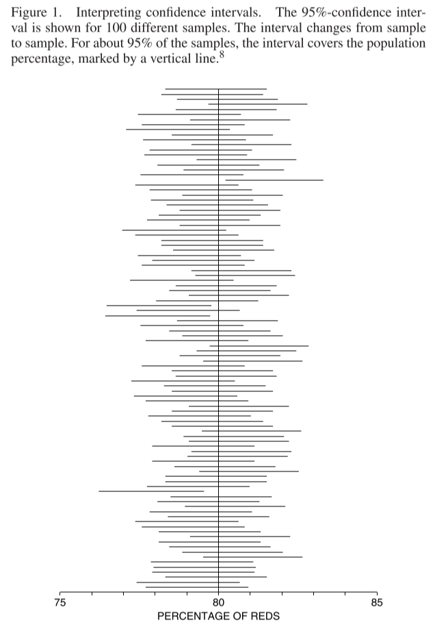
The chapter introduces confidence intervals, using standard errors esimated from the data plus the normal approximation. The chapter gives a frequentist interpretation:
In example 1 on p. 378, a simple random sample was taken to estimate the percentage of students registered at a university in fall 2005 who were living at home. An approximate 95% - confidence interval for this percentage ran from 75% to 83% . . . It seems more natural to say “There is a 95% chance that the population percentage is between 75% and 83%.” But there is a problem here. In the frequency theory, a chance represents the percentage of the time that something will happen. No matter how many times you take stock of all the students registered at that university in the fall of 2005, the percentage who were living at home back then will not change. Either this percentage was between 75% and 83%, or not. There really is no way to define the chance that the parameter will be in the interval from 75% to 83%. That is why statisticians have to turn the problem around slightly. They realize that the chances are in the sampling procedure, not in the parameter. And they use the new word “confidence” to remind you of this.
Here’s a nice figure that illustrates this interpretation:
The chapter includes a caveat:
The methods of this chapter were developed for simple random samples. They may not apply to other kinds of samples. Many survey organizations use fairly complicated probability methods to draw their samples (section 4 of chapter 19). As a result, they have to use more complicated methods for estimating their standard errors . . . Here is the reason. Logically, the procedures in this chapter all come out of the square root law (section 2 of chapter 17). When the size of the sample is small relative to the size of the population, taking a simple random sample is just about the same as drawing at random with replacement from a box — the basic situation to which the square root law applies. The phrase “at random” is used here in its technical sense: at each stage, every ticket in the box has to have an equal chance to be chosen. If the sample is not taken at random, the square root law does not apply, and may give silly answers.
The Gallup poll, for instance, does not use simple random sampling, and in 11 of the 14 elections between 1952 and 2004 the error was considerably larger than the SE for a simple random sample. Chapter 19 described some of the issues pollsters face.