Chapter 9 More About Correlation

9.1 Chapter Notes

Some facts about correlation:

• Because of the way Pearson’s r is calculated (by first standardising both variables), it is not affected by changes of scale.
• It is symmetric; the correlation between x and y is the same as the correlation between y and x.
• Because correlation is calculated by conversion to standard units (including dividing by SDs). Two sets of paired variables can have the same correlation, but very different standard deviations and therefore very different-looking plots. This image is great, I think:

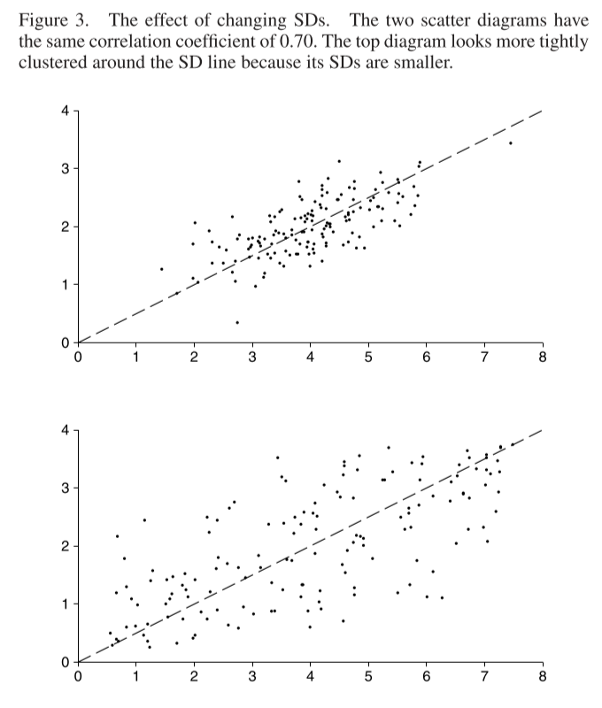
To compare corellations like-for-like graphically, the horizontal standard deviations should take up the same space on the page for both graphs, and likewise for the vertical SDs.

Here’s some detail about rough distance points will appear above or below the SD line.

If r is close to 1, then a typical point is only a small fraction of a vertical SD above or below the SD line. If r is close to 0, then a typical point is above or below the line by an amount roughly comparable in size to the vertical SD. The connection between the correlation coefficient and the typical distance above or below the SD line can be expressed mathematically, as follows. The r.m.s. vertical distance to the SD line equals

\[ \sqrt{2(1-|r|)} \times\text{the vertical SD} \]

Take, for example, a correlation of 0.95. Then

\[ \sqrt{2(1-|r|)} = \sqrt{0.1} \approx 0.3 \]

So the spread around the SD line is about 30% of a vertical SD. That is why a scatter diagram with r = 0.95 shows a fair amount of spread around the line.

Outliers and Non-Linearity

Outliers and non-linearity are problem cases. In both the graphs below, the variables show a strong association, but r is near 0.In the first case because of the single outlier point, in the second because of the non-linearity. This means that Pearson’s r is not an appropriate tool to summarise these variables. It does not mean, for example, that the outlier should be thrown away, unless there is a principled reason why it is inappropriate to include it.

Pearson’s r measures linear association, not association in general.

Ecological Correlations.

Ecological correlations are based on rates or averages. They are often used in political science and sociology. And they tend to over-state the strength of an association. So watch out.

Here is another example. From Current Population Survey data for 2005, you can compute the correlation between income and education for men age 25–64 in the United States: r ≈ 0.42. For each state (and D.C.), you can compute average educational level and average income. Finally, you can compute the correlation between the 51 pairs of averages: r ≈ 0.70. If you used the correlation for the states to estimate the correlation for the individuals, you would be way off. The reason is that within each state, there is a lot of spread around the averages.