Chapter 8 Correlation
8.1 Chapter Notes
Now instead of looking at the distribution of a single variable, we begin studying the relationship between two variables.
Scatter diagram for heights of fathers and their sons at maturity, collected by Karl Pearson.
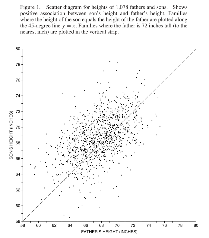
We can summarise this scatter plot using the average of the x and y values, and also their standard deviations. But that doesn’t tell us about the strength of the associtation between the two variables.
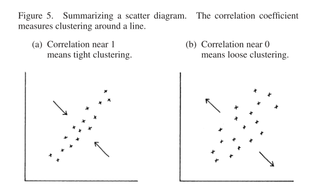
Both of the above clouds have the same centre (x,y average) and the same spread both horizontally and vertically. To measure the association, we need the correlation coefficient.
The SD line - the SD line goes through the point of averages, and through all the points that are an equal number of standard deviations away from the average for both variables. Interesting, I don’t think I’ve come across the concept of an SD line before, I wonder how it’s related to e.g. the OLS regression lines. Some discussion in this Stats Stack Exchange question.
Here is how to compute the (Pearson) correlation coefficient:
Convert each variable to standard units. The average of the products gives the correlation coefficient.
I.e. the process is like this:
- Begin with a set of paired data, x and y variables.
- Convert the x variable to standard units - subtract the average and divide by the standard deviation.
- Repeat with the y variable.
- For each pair, compute the product.
- Take the average of the products.
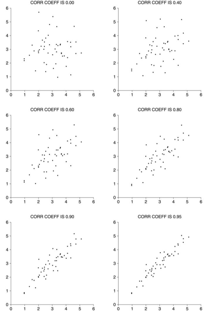
Why does this work as a measure of linear association? The description in the chapter gives a little intuition - we can imagine plotting a scatter plot of the variables, converted into standard units. If we carve the plot into four quadrants, points in the upper right quadrant will have both variables above the average, multiplying them will give a positive number. Similarly points in the bottom left quadrant will be both negative and their product a positive number. The products for points in the other two products will be negative. It’s also easy to show that a perfect correlation implies \(r=1\) by just plugging in the definitions.
This gives a sense of how this figure can work as a measure of association, but it’s not wholly satisfactory.
Here’s another way to compute Pearson’s r:
\[ r = \frac{\text{cov}(x,y)}{(\text{SD of }x) \times (\text{SD of }y)} \]
where
\[ \text{cov}(x,y) = (\text{average of products }xy) - (\text{average of }x) \times (\text{average of }y). \]