Chapter 24 A Model for Measurement Error

24.1 Chapter Notes

This chapter applies our box models (or chance models or stochastic models) to the study of measurement error.

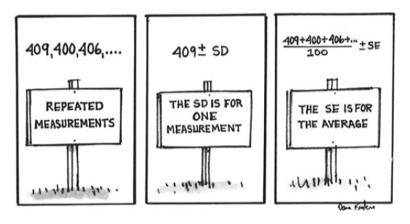
In chapter six we used the SD as a measure of the likely size of the chance error in a single measurement. In this chapter we compute the likely chance error of the average of the estimates. We use:

\[ \begin{aligned} \text{SE for the average} &= \frac{\text{SE of the sum}}{\text{number of measurements}} \\ &=\frac{\sqrt{\text{number of measurements}}\times \text{SD of the sample}}{\text{number of measurements}}\\ &=\frac{ \text{SD of the sample}}{\sqrt{\text{number of measurements}}}=\frac{\sigma}{\sqrt{n}} \end{aligned} \] Here we have again used the SD of the sample as a stand-in for the SD of the population.

When the normal approximation applies, we can use that to construct confidence intervals.

A nice historical example:

There is a connection between the theory of measurement error and neon signs. In 1890, the atmosphere was believed to consist of nitrogen (about 80%), oxygen (a little under 20%), carbon dioxide, water vapor—and nothing else. Chemists were able to remove the oxygen, carbon dioxide, and water vapor. The residual gas should have been pure nitrogen.

Lord Rayleigh undertook to compare the weight of the residual gas with the weight of an equal volume of chemically pure nitrogen. One measurement on the weight of the residual gas gave 2.31001 grams. And one measurement of the pure nitrogen gave a bit less, 2.29849 grams. However, the difference of 0.01152 grams was rather small, and in fact was comparable to the chance errors made by the weighing procedure.

Could the difference have resulted from chance error? If not, the residual gas had to contain something heavier than nitrogen. What Rayleigh did was to replicate the experiment, until he had enough measurements to prove that the residual gas from the atmosphere was heavier than pure nitrogen.

He went on to isolate the rare gas called argon,which is heavier than pure nitrogen and present in the atmosphere in small quantities. Other researchers later discovered the similar gases neon, krypton, and xenon, all occurring naturally (in trace amounts) in the atmosphere. These gases are what make “neon” signs glow in different colors.

An endnote points to Youden’s ‘Experimentation and Measurement’ for this example.

The chapter describes a box model for measurement error it calls ‘the Gauss model’:

In the Gauss model, each time a measurement is made, a ticket is drawn at random with replacement from the error box. The number on the ticket is the chance error. It is added to the exact value to give the actual measurement. The average of the error box is equal to 0.

The SD of the box is usually unknown and must be estimated from the data.

When the Gauss model applies, the SD of a series of repeated measurements can be used to estimate the SD of the error box. The estimate is good when there are enough measurements.

And again the chapter warns about making assumptions that underpin the box model when those assumptions are not justified:

Statistical inference can be justified by putting up an explicit chance model for the data. No box, no inference.