Chapter 28 The Chi-Square Test
28.1 Chapter Notes
The \(\chi^2\)-test is used when we have more than two categories. The chapter uses the example of a test to check whether a die is fair.
Here’s a table of what we observe on 60 rolls of the die, against what we expect:
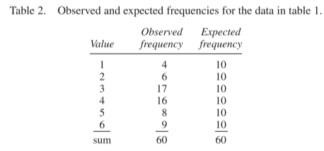
Here we can see that there are too many 3’s. The standard error for the number of 3’s is \(\sqrt{60} \times \sqrt{1/6 \times 5/6} \approx 2.9\). So the observed number 17 is about 2.4 SEs above the expected value.
But we shouldn’t conclude yet that the die is not fair. The more lines in the table, the higher the probability that one of them will look suspicious even with a fair die. We need to take the data all together, and this what the \(\chi^2\)-test allows.
\[ \chi^2 = \sum\frac{(\text{observed frequency} - \text{expected frequency})^2}{\text{expected frequency}} \] Large values indicate that the observed frequencies are far from the expected ones. Small values indicate that the observed frequencies are close to the expected ones (the Fisher example below gives an example of a case where the \(\chi^2\)-test is used to show that observed frequencies are too close to the expected ones). Here’s the calculation for the table above:

Now we need the probability of observing a \(\chi^2\)-statistic of 14.2 or more, given a fair die is rolled 60 times.
The \(\chi^2\) distribution, has one parameter - degrees of freedom. With a fully specified model (no parameters to estimate) as in this case, the degrees of freedom are given by
\[ \text{degrees of freedom} = \text{number of terms in } \chi^2 - \text{one} \] In this case \(6 - 1 = 5\).
Here’s how we calculate the amount of probability mass at and above 14.2 for a \(\chi^2\) curve with 5 degrees of freedom:
pchisq(14.2, 5,lower.tail = FALSE)## [1] 0.01438768I.e. 1.4%. This is our p-value.
We use a \(\chi^2\)-test when it matters how many tickets of each kind are in the box. If we only care about averages, we can use the z-test.
A summary:
- The \(\chi^2\)-test says whether the data are like the result of drawing at random from a box whose contents are given.
- The z-test says whether the data are like the result of drawing at random from a box whose average is given.
Whatever is in the box, the same \(\chi^2\)-curves and tables can be used to approximate P,provided N is large enough. That is what motivated the formula. With other test statistics, a new curve would be needed for every box.
There is then a section in the chapter about how Fisher used the \(\chi^2\)-test to evaluate Mendel’s data, concluding that the data was manipulated.
The important point here is that Fisher could combine the results of more than one experiment and calculate a single \(\chi^2\)-statistic for the overall probability of the data, given the hypothesis that the experiments were conducted as described.
With independent experiments, the results can be pooled by adding up the separate \(\chi^2\)-statistics; the degrees of freedom add up too.
The other difference here is that the left tail area of the appropriate \(\chi^2\) curve must be used. This is because small values of \(\chi^2\) say that the observed frequencies are closer to the expected ones than chance would allow which is the alternative hypothesis in this case.
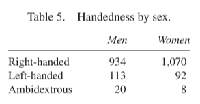
The \(\chi^2\)-statistic can also be used when testing for independence. An example in the chapter concerns handedness and sex. Are they independent? Here’s a table:
We can analyse this example using a box with six types of tickets:
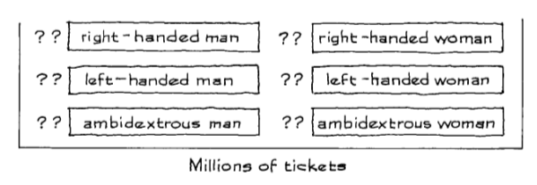
The composition of the box is unknown, and so we have 6 parameters to estimate.
To calculate our statistic, we need to compare the observed figures in the table above to the expected frequencies:
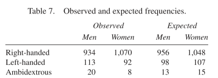
\[ \begin{aligned} \chi^2 &= \sum\frac{(\text{observed frequency} - \text{expected frequency})^2}{\text{expected frequency}}\\ &= \frac{(934-956)^2}{956} + \frac{(1070-1048)^2}{1048} \\ &+ \frac{(113-98)^2}{98} +\frac{(92-107)^2}{107} \\ &+ \frac{(20-13)^2}{13} +\frac{(8-15)^2}{15} \\ &\approx 12 \end{aligned} \] When testing independence in an \(m \times n\) table, there are \((m-1) \times (n-1)\) degrees of freedom. To see notice that there are 22 fewer right-handed men than expected in the table above, and there are 22 more right-handed women. Once you know one figure, you know the other because the differences must add up to zero horizontally. So we only need to know \((n-1)\) of the columns. We only need to know \((m-1)\) of the rows, because the differences must also add up to zero vertically. We have 22 fewer right-handed men than expected, which means we must have 22 more left-handed and ambidextrous men.
So where did the expected frequencies in the above table come from?
To start with, we compute the row and column totals:
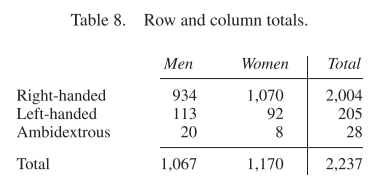
We can see that
\[ \frac{2004}{2237} = 89.6\% \] of our sample are right-handed. If handedness and sex were independent we would expect 89.6% of men to be right-handed. We expect \(89.4\% \times 1067 \approx 956\) right-handed men.
We should be computing the expected frequencies directly from the box model, but we don’t know the box composition. We instead estimate expected frequencies from the sample and the assumption of independence. The chapter says that “estimated expected frequencies” would be the more appropriate term.